EarthCare ATLID Analysis

import xarray as xr
import numpy as np
import matplotlib.pyplot as plt
import matplotlib.colors as colors
from scipy.interpolate import interp1d
from matplotlib.colors import ListedColormap, BoundaryNorm

# ========================================================================================================================
#                                         Variable "particle_extinction_coefficient_355nm"
# ========================================================================================================================

# Uncomment if running on CoLab
##!pip install netCDF4

# Uncomment if running on CoLab
##import pathlib
##from pathlib import Path
##import gdown

##DATA_LINK = "1Ek1YxH1qWZb4FRDF81vJhiqwL8mSnWhj"
##CREATE_BASE = pathlib.Path("./sample_data")
##CREATE_BASE.mkdir(parents=True, exist_ok=True)
##gdown.download(id=DATA_LINK, output=str(CREATE_BASE / "ECA_EXBC_ATL_EBD_2A_20260303T143905Z_20260303T162808Z_10015D.h5"), quiet=False)

# Step 1. Read file

file_path = "./sample_data/ECA_EXBC_ATL_EBD_2A_20260303T143905Z_20260303T162808Z_10015D.h5"

ds = xr.open_dataset(
    file_path,
    engine="h5netcdf",
    group="ScienceData")

# Step 2. Use variables

lat = ds["latitude"].values
lon = ds["longitude"].values
time = ds["time"].values
elevation = ds["elevation"].values
height = ds["height"].values

ext = ds["particle_extinction_coefficient_355nm"].values
depol = ds["particle_linear_depol_ratio_355nm"].values # NumPy array (data only)
depol_da   = ds["particle_linear_depol_ratio_355nm"] # xarray DataArray (data + metadata)
quality = ds["quality_status"].values
simple_class = ds["simple_classification"].values

# Step 3. Print unit and fill values
# See what the measurement unit is and if there are any fill values in the file

ext_da = ds["particle_extinction_coefficient_355nm"]

fill_value = ext_da.attrs.get("_FillValue", None)
units = ext_da.attrs.get("units", "unknown")

print("Extinction units:", units)
print("Fill value:", fill_value)

# Step 4. Location
# Badajoz, also an AERONET station

target_lat = 38.8803 
target_lon = -6.9753
radius_km = 50.0

# Step 5. Haversine distance
#The Haversine formula computes the distance between the target point and long/lat with every EarthCARE profile location

def haversine(lat0, lon0, lat, lon):

    r = 6371.0

    lat0 = np.radians(lat0)
    lon0 = np.radians(lon0)

    lat = np.radians(lat)
    lon = np.radians(lon)

    dlat = lat - lat0
    dlon = lon - lon0

    a = (
        np.sin(dlat / 2.0) ** 2
        + np.cos(lat0)
        * np.cos(lat)
        * np.sin(dlon / 2.0) ** 2)

    return 2 * r * np.arcsin(np.sqrt(a))

# Step 6. Select location-relevant profiles

distance = haversine(
    target_lat,
    target_lon,
    lat,
    lon)

mask = distance <= radius_km     #50km

if not np.any(mask):
    raise ValueError(
        f"No profiles found within {radius_km} km.")

# Subset

sub_lat = lat[mask]
sub_lon = lon[mask]
sub_time = time[mask]

sub_ext = ext[mask, :]
sub_height = height[mask, :]
sub_quality = quality[mask, :]

print(f"Profiles selected: {sub_ext.shape[0]}")

# Step 7. Handle fill values, turning them into NANs

if fill_value is not None:
    sub_ext = np.where(
        sub_ext == fill_value,
        np.nan,
        sub_ext)

# Step 8. Quality filtering, keeping bins with GOOD_FLAG

GOOD_FLAG = 0

sub_ext = np.where(
    sub_quality == GOOD_FLAG,
    sub_ext,
    np.nan)

# Step 9. Common altitude grid
#Create a common altitude grid and interpolate every profile onto this exact grid.

alt_grid = np.arange(
    500,
    10001,
    100)

n_profiles = sub_ext.shape[0]

ext_interp = np.full(
    (n_profiles, len(alt_grid)),
    np.nan)

for i in range(n_profiles):

    z = sub_height[i, :]
    e = sub_ext[i, :]

    valid = (
        np.isfinite(z)
        & np.isfinite(e))

    if valid.sum() < 5:
        continue

    f = interp1d(
        z[valid],
        e[valid],
        bounds_error=False,
        fill_value=np.nan)

    ext_interp[i, :] = f(alt_grid)

# Step 10. Statistics: mean, standard deviation, number of valid observations, standard error

mean_profile = np.nanmean(
    ext_interp,
    axis=0)

std_profile = np.nanstd(
    ext_interp,
    axis=0)

n_valid = np.sum(
    np.isfinite(ext_interp),
    axis=0)

stderr_profile = (
    std_profile /
    np.sqrt(np.maximum(n_valid, 1)))

start_time = np.min(sub_time)
end_time   = np.max(sub_time)
duration_minutes = (
    (end_time - start_time)
    / np.timedelta64(1, "m"))

print("Number of profiles:", n_profiles)
print(
    "Altitude range:",
    alt_grid.min(),
    alt_grid.max(),
    "m")
print(
    "Mean extinction:",
    np.nanmin(mean_profile),
    np.nanmax(mean_profile))
print(f"Start time (UTC): {start_time}")
print(f"End time (UTC): {end_time}")
print(f"Duration: {duration_minutes:.2f} minutes")

# Step 11. Plot profiles

fig, ax = plt.subplots(
    figsize=(5, 8))

# Convert altitude to km
alt_km = alt_grid / 1000.0

# Mean profile
ax.plot(
    mean_profile,
    alt_km,
    lw=2,
    label="Mean extinction")

# Standard error envelope
ax.fill_betweenx(
    alt_km,
    mean_profile - stderr_profile,
    mean_profile + stderr_profile,
    alpha=0.3,
    label="95% confidence region")

ax.set_xlabel(
    f"Particle Extinction Coefficient 355 nm ({units})")
ax.set_ylabel(
    "Altitude (km)")
ax.set_title(
    f"EarthCARE Mean Extinction Profile\n"
    f"{n_profiles} profiles within {radius_km:.0f} km")
ax.grid(True, alpha=0.3)
ax.set_ylim(0.5, 10)
ax.legend()

plt.tight_layout()

plt.savefig(
    "EarthCARE_mean_profile_Badajoz.png",
    dpi=300,
    bbox_inches="tight")

plt.show()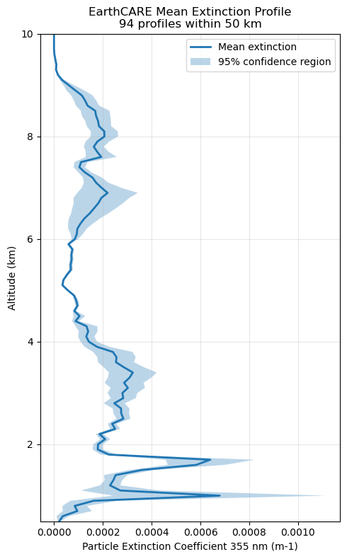

# Step 12. Plot Curtain Plot

# Calculate cumulative distance along the track for the X-axis
# This makes the plot more physically meaningful than just "Profile Index"
track_distances = [0]
for i in range(1, len(sub_lat)):
    d = haversine(sub_lat[i-1], sub_lon[i-1], sub_lat[i], sub_lon[i])
    track_distances.append(track_distances[-1] + d)
track_distances = np.array(track_distances)

fig, ax = plt.subplots(figsize=(12, 5))

# Create a meshgrid for plotting
# X: cumulative distance, Y: altitude in km
X, Y = np.meshgrid(track_distances, alt_grid / 1000.0)

# Transpose ext_interp to match (height, distance) shape
# We use LogNorm because lidar extinction often spans several orders of magnitude
mesh = ax.pcolormesh(
    X, Y, 
    ext_interp.T, 
    shading='auto',
    cmap='viridis',
    norm=colors.LogNorm(vmin=1e-6, vmax=1e-2) # Adjust limits based on your data
)

# Add Colorbar
cbar = fig.colorbar(mesh, ax=ax, extend='both')
cbar.set_label(f"Extinction [{units}]")

# Labels and Titles
ax.set_xlabel("Distance along track (km)")
ax.set_ylabel("Altitude (km)")
ax.set_title(
    f"EarthCARE Extinction Curtain\n"
    f"Target: {target_lat}, {target_lon} | Radius: {radius_km}km"
)

# Add a secondary X-axis at the top to show Latitude
ax2 = ax.twiny()
ax2.set_xlim(ax.get_xlim())
tick_indices = np.linspace(0, len(sub_lat) - 1, 5, dtype=int)
ax2.set_xticks(track_distances[tick_indices])
ax2.set_xticklabels([f"{sub_lat[i]:.2f}N" for i in tick_indices])
ax2.set_xlabel("Latitude")

ax.set_ylim(0, 10) # Set height limit to 10km
ax.grid(True, alpha=0.2, color='white')

plt.tight_layout()
plt.savefig(
    "EarthCARE_extinction_curtain.png",
    dpi=300,
    bbox_inches="tight",
    pad_inches=0.05
)


plt.show()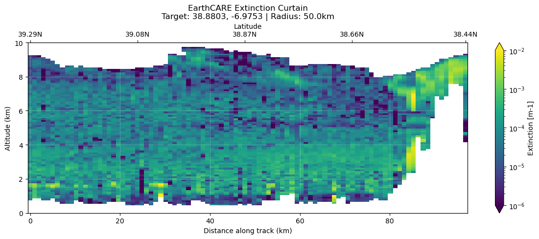

# ========================================================================================================================
#                                         Variable "particle_linear_depol_ratio_355nm"
# ========================================================================================================================

# Step 2. Inspect depol metadata

fill_depol = depol_da.attrs.get("_FillValue", None)
units_depol = depol_da.attrs.get("units", "1")   # dimensionless ratio
print("Depol units:", units_depol)
print("Depol fill value:", fill_depol)
print("Depol range in file:", np.nanmin(depol), "–", np.nanmax(depol))

# Step 3. Haversine (similar to extinction variable)

def haversine(lat0, lon0, lat, lon):
    r = 6371.0
    lat0, lon0, lat, lon = map(np.radians, [lat0, lon0, lat, lon])
    dlat = lat - lat0
    dlon = lon - lon0
    a = np.sin(dlat/2)**2 + np.cos(lat0)*np.cos(lat)*np.sin(dlon/2)**2
    return 2 * r * np.arcsin(np.sqrt(a))

# Step 4. Spatial selection and number of available profiles

target_lat = 38.8803
target_lon = -6.9753
radius_km  = 50.0

distance = haversine(target_lat, target_lon, lat, lon)
mask = distance <= radius_km
if not np.any(mask):
    raise ValueError(f"No profiles found within {radius_km} km.")

sub_lat    = lat[mask]
sub_lon    = lon[mask]
sub_time   = time[mask]
sub_ext    = ext[mask, :]
sub_depol  = depol[mask, :]
sub_height = height[mask, :]
sub_quality = quality[mask, :]
print(f"Profiles selected: {sub_ext.shape[0]}")

# Step 5. Fill value masking

ext_da     = ds["particle_extinction_coefficient_355nm"]
fill_ext   = ext_da.attrs.get("_FillValue", None)

if fill_ext is not None:
    sub_ext = np.where(sub_ext == fill_ext, np.nan, sub_ext)
if fill_depol is not None:
    sub_depol = np.where(sub_depol == fill_depol, np.nan, sub_depol)

# Step 6. Quality filtering (keep GOOD_FLAG = 0 only, check EBD documentation for details)

GOOD_FLAG = 0
sub_ext   = np.where(sub_quality == GOOD_FLAG, sub_ext,  np.nan)
sub_depol = np.where(sub_quality == GOOD_FLAG, sub_depol, np.nan)

# Sanity clamp: depol is a ratio in [0, 1]; clip unphysical values
sub_depol = np.where((sub_depol >= 0) & (sub_depol <= 1), sub_depol, np.nan)

# Step 7. Interpolate both variables onto common altitude grid

alt_grid   = np.arange(500, 10001, 100)   # 500 m – 10 000 m, 100 m bins
n_profiles = sub_ext.shape[0]

ext_interp   = np.full((n_profiles, len(alt_grid)), np.nan)
depol_interp = np.full((n_profiles, len(alt_grid)), np.nan)

for i in range(n_profiles):
    z = sub_height[i, :]
    e = sub_ext[i, :]
    d = sub_depol[i, :]

    valid_e = np.isfinite(z) & np.isfinite(e)
    valid_d = np.isfinite(z) & np.isfinite(d)

    if valid_e.sum() >= 5:
        ext_interp[i, :]   = interp1d(z[valid_e], e[valid_e],
                                       bounds_error=False, fill_value=np.nan)(alt_grid)
    if valid_d.sum() >= 5:
        depol_interp[i, :] = interp1d(z[valid_d], d[valid_d],
                                       bounds_error=False, fill_value=np.nan)(alt_grid)

# Step 8. Profile statistics

def profile_stats(arr):
    mean   = np.nanmean(arr, axis=0)
    std    = np.nanstd(arr, axis=0)
    n      = np.sum(np.isfinite(arr), axis=0)
    stderr = std / np.sqrt(np.maximum(n, 1))
    return mean, std, n, stderr

mean_ext,   _, _, stderr_ext   = profile_stats(ext_interp)
mean_depol, _, _, stderr_depol = profile_stats(depol_interp)

# Step 9. Plot Mean depolarisation vertical profile

alt_km = alt_grid / 1000.0

fig, ax = plt.subplots(figsize=(5, 8))
ax.plot(mean_depol, alt_km, color="darkorange", lw=2, label="Mean δ_p")
ax.fill_betweenx(alt_km,
                 mean_depol - stderr_depol,
                 mean_depol + stderr_depol,
                 alpha=0.3, color="darkorange", label="±1 SE")
ax.set_xlabel("Particle Linear Depolarisation Ratio 355 nm (–)")
ax.set_ylabel("Altitude (km)")
ax.set_title(f"EarthCARE ATLID Mean Depolarisation Profile\n"
             f"{n_profiles} profiles within {radius_km:.0f} km")
ax.set_xlim(0, 0.5)   # physical range; widen if data demands it
ax.set_ylim(0.5, 10)
ax.grid(True, alpha=0.3)
ax.legend()
plt.tight_layout()
plt.savefig("EarthCARE_depol_profile.png", dpi=300, bbox_inches="tight")
plt.show()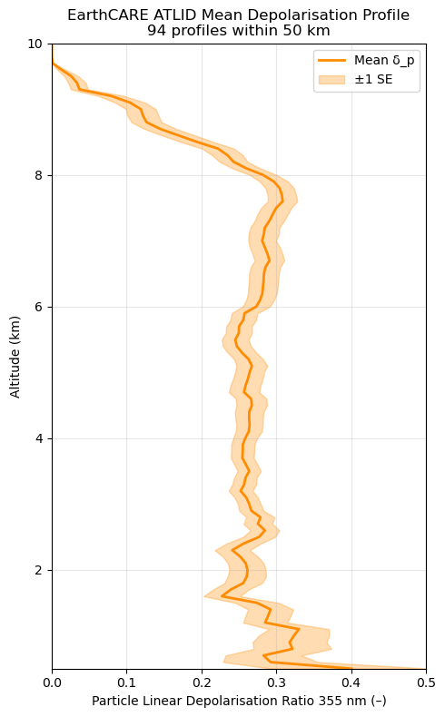

# Step 10. Plot Depolarisation curtain plot

track_distances = [0]
for i in range(1, len(sub_lat)):
    d = haversine(sub_lat[i-1], sub_lon[i-1], sub_lat[i], sub_lon[i])
    track_distances.append(track_distances[-1] + d)
track_distances = np.array(track_distances)

X, Y = np.meshgrid(track_distances, alt_km)

fig, ax = plt.subplots(figsize=(12, 5))
mesh = ax.pcolormesh(X, Y, depol_interp.T,
                     shading="auto",
                     cmap="RdYlBu_r",       # red = high depol (dust/ice), blue = low (spherical)
                     vmin=0, vmax=0.4)       # linear scale — depol is already bounded
cbar = fig.colorbar(mesh, ax=ax, extend="max")
cbar.set_label("Particle Linear Depolarisation Ratio δ_p (–)")

ax.set_xlabel("Distance along track (km)")
ax.set_ylabel("Altitude (km)")
ax.set_title(f"EarthCARE ATLID Depolarisation Curtain\n"
             f"Target: {target_lat}°N, {target_lon}°E | Radius: {radius_km:.0f} km")
ax.set_ylim(0, 10)
ax.grid(True, alpha=0.2, color="white")

ax2 = ax.twiny()
ax2.set_xlim(ax.get_xlim())
tick_idx = np.linspace(0, len(sub_lat) - 1, 5, dtype=int)
ax2.set_xticks(track_distances[tick_idx])
ax2.set_xticklabels([f"{sub_lat[i]:.2f}°N" for i in tick_idx])
ax2.set_xlabel("Latitude")

plt.tight_layout()
plt.savefig("EarthCARE_depol_curtain.png", dpi=300, bbox_inches="tight")
plt.show()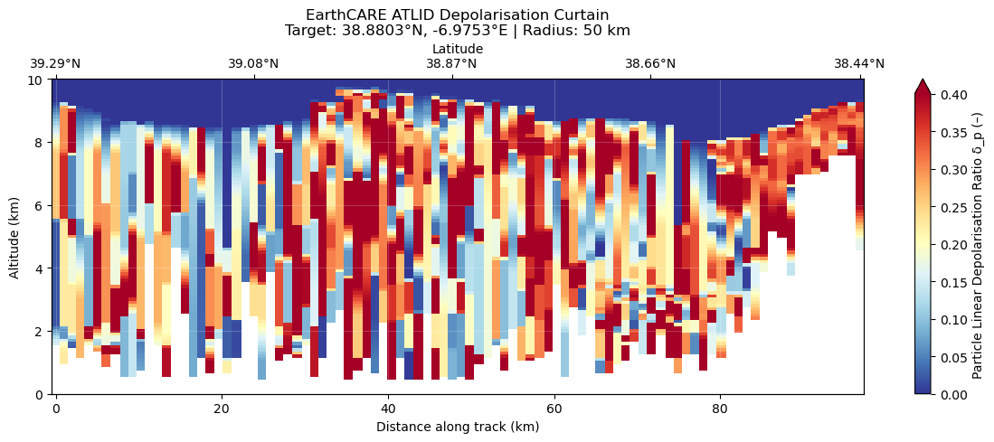

# ========================================================================================================================
#                                         Variable "simple_classification"
# ========================================================================================================================

sub_class = simple_class[mask, :]

# Define class labels
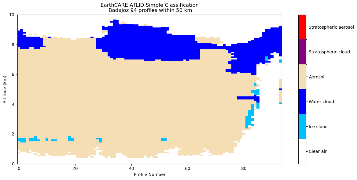
class_labels = {
     0: "Clear air",
     1: "Ice cloud",
     2: "Water cloud",
     3: "Aerosol",
     4: "Stratospheric cloud",
     5: "Stratospheric aerosol"}

colors = [
    "white",       #  0 Clear
    "deepskyblue", #  1 Ice
    "blue",        #  2 Water
    "wheat",      #  3 Aerosol
    "purple",      #  4 Stratospheric cloud
    "red"]          #  5 Stratospheric aerosol

cmap = ListedColormap(colors)
norm = BoundaryNorm(
    np.arange(-0.5, len(colors)+0.5),
    cmap.N)

# Plot curtain
fig, ax = plt.subplots(figsize=(12,6))

pcm = ax.pcolormesh(
    np.arange(sub_class.shape[0]),
    sub_height.T / 1000.0,
    sub_class.T,
    shading="auto",
    cmap=cmap,
    norm=norm)

cbar = plt.colorbar(
    pcm,
    ticks=list(class_labels.keys()))

cbar.ax.set_yticklabels(
    [class_labels[k] for k in class_labels])

ax.set_xlabel("Profile Number")
ax.set_ylabel("Altitude (km)")

ax.set_title(
    f"EarthCARE ATLID Simple Classification\n Badajoz "
    f"{sub_class.shape[0]} profiles within {radius_km:.0f} km")

ax.set_ylim(0,10)

plt.tight_layout()

plt.savefig(
    "EarthCARE_simple_classification.png",
    dpi=300,
    bbox_inches="tight",
    pad_inches=0.05)

plt.show()